- The field of statistics involves methods for:
- 1.Designing and carrying out research studies.
- 2.Describing collected data.
- 3.Making decisions, predictions, or inferences about phenomena represented by the data by designing valid experiments and drawing reliable conclusions.
- Branches of Statistics
- Descriptive statistics: Gives numerical and graphic procedures to summarize a collection of data in a clear and understandable way
- Inferential statistics: statistical methods that generalize results from a sample to a population.
Descriptive Measures
- Measures of Central Tendency. They are computed to give a “center” around which the measurements in the data are distributed.
- Measures of Variation or Variability. They describe “data spread” or how far away the measurements are from the center.
- Measures of Relative Standing. They describe the relative position of specific measurements in the data.
Arithmetic mean
This is the most popular and useful measure of central location
MEAN= Sum of the measurements / Number of measurements
Sample mean: 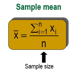
Population mean. 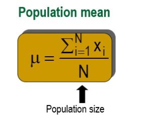
The median
The median of a set of measurements is the value that falls in the middle when the measurements are arranged in order of magnitude.
Example
Seven employee salaries were recorded
(in 1000s) : 28, 60, 26, 32, 30, 26, 29.
Find the median salary.
Suppose one employee’s salary of $31,000
was added to the group recorded before.
Find the median salary.
Odd Number Observations
First, sort the salaries.
Then, locate the value
in the middle
26, 26, 28, 29, 30, 32, 60
Even Number Observation
First, sort the salaries.
Then, locate the values
in the middle
26,26,28,29,29.5,30,32,60,31
The mode
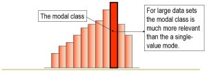
- The mode of a set of measurements is the value that occurs most frequently.
- Set of data may have one mode (or modal class), or two or more modes.
Example
- The following are temperature readings: : 31, 34, 36, 33, 28, 34, 30, 34, 32, 40.
- The mode of this data set is 34 in.
Shapes of Distributions
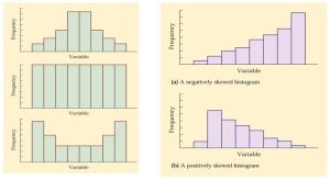
- A Distribution is perfectly symmetric if its right half is a mirror image of its left half.
- Distributions that are not symmetric are referred to as skewed.
- A Distribution with a long right-hand tail is said to be skewed to the right, or positively skewed.
- A histogram with a long left-hand tail is said to be skewed to the left, or negatively skewed.
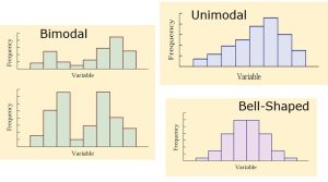
- A Distributions is unimodal if it has only one peak, or mode, and bimodal if it has two clearly distinct modes. In principle, a distribution can have more than two modes, but this does not happen often in practice.
Shapes of Distributions
Shapes of Distributions
Relationship among Mean, Median, and Mode
- If a distribution is symmetrical, the mean, median and mode coincide

-
If a distribution is non symmetrical, and skewed
to the left or to the right, the three measures
differ.
A positively skewed distribution
(“skewed to the right”) 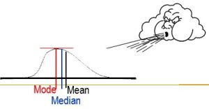
- If a distribution is symmetrical, the mean, median and mode coincide
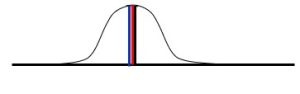
- If a distribution is non symmetrical, and skewed to the left or to the right, the three measures differ.
Measures of variability
(Looking beyond the average)
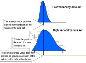
- Measures of central tendency fail to tell the whole story about the distribution.
- A question of interest still remains unanswered:
How typical is the average value of all the measurements in the data set?
or
How much spread out are the measurements about the average value?
Observe two hypothetical data sets
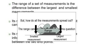
The range
The variance
- This measure of dispersion reflects the values of all the measurements.
- The variance of a sample of n measurements x1, x2, …,xn having a mean is defined as

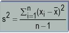
The standard deviation of a set of measurements is the square root of the variance of the measurements.
Example
Percentage change in salinity over the last 10 years for two wells are shown below. Which one have a higher dispersion?
Well A: 8.3, -6.2, 20.9, -2.7, 33.6, 42.9, 24.4, 5.2, 3.1, 30.05
Well B: 12.1, -2.8, 6.4, 12.2, 27.8, 25.3, 18.2, 10.7, -1.3, 11.4
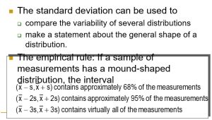
Interpreting Standard Deviation
Measures of Relative Standing
Percentile
The pth percentile of a set of measurements is the value for which
- at most p% of the measurements are less than that value
- at most 100(1-p)% of all the measurements are greater than that value.
Example
Suppose 600 is the 78% percentile of a GMAT score. Then
For any data
- At least 75% of the measurements differ from the mean less than twice the standard deviation.
- At least 89% of the measurements differ from the mean less than three times the standard deviation.
Note: This is a general property and it is called Tchebichev’s Rule: At least 1-1/k2 of the observation falls within k standard deviations from the mean. It is true for every dataset.
Example of Tchebichev’s Rule
Suppose that for a certain data is :
- Mean = 20
- Standard deviation =3
Then:
- A least 75% of the measurements are between 14 and 26
- At least 89% of the measurements are between 11 and 29
Examining Relationships
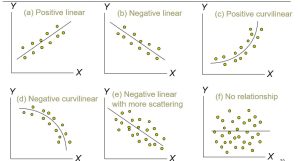
In any graph of data, look for the overall pattern and for striking deviations from that pattern.
You can describe the overall pattern by the:
- Form: Describe the type of trend between X and Y (linear, quadratic, exponential).
- Direction: describes the direction of the trend upward (positive) or downward (negative).
- Strength: Measures the amount of scatter around the general trend.
An important kind of deviation is an outlier, an individual that falls outside the overall pattern of the relationship.
Examples
Correlation Coefficient
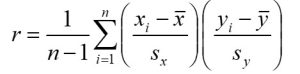
- The coefficient of correlation is a measure of the strength of linear association between two variables, x and y;
- In Minitab:
- Stat → Basic Statistics → Correlation
- (variables Y X) → ok
Properties of r
- -1 ≤ r ≤ 1.
- If r < 0 à negative linear association
- If r > 0 à positive linear association
- r is independent of units.
- Empirical rule to interpret r:
- 0 < |r| ≤ 0.5 à weak linear association
- 0.5 < |r| ≤ 0.8 à moderate linear association
- 0.8 < |r| ≤ 1 à strong linear association.
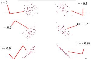
- Scatters and correlations
Forecasting and Time Series
l
Forecasting is predicting the future events.
Examples:
- What will be the unemployment rate next year?
- Is there a trend in global temperature?
- What is the seasonal effect?
- Forecasting is not an exact science but instead consists of a set of statistical tools and techniques which are supported by human judgment and intuition.
- Forecasters rely on past data on the assumption that the pattern that has been identified will continue in the future.
Time Series Data
- A time series is a set of chronologically ordered points of data.
- In a time series the sequence of the observations is important, in contrast to cross-sectional data for which the sequence of observations is not important.
- We are mainly interested in discrete-time time series with equally fixed time intervals. e.g. observations made daily, weekly, monthly, etc.
Examples:
Economic indicators: Sales figures, employment statistics, stock market indices, …
Meteorological data: precipitation, temperature,…
Example
Records of a person’s height:
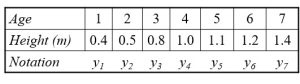
For this example, we have n=7 observations.
We denote the observation at time t by yt. The time series can be written as
{0.4, 0.5, 0.8, 1.0, 1.1, 1.2, 1.4}